library(tidyverse)
library(pracma)BrainChart calibration tutorial
Introduction
The code in this repository extends the original BrainChart codebase, and therefore can’t be assembled into a standard R package without restructuring that code.
First, load the libraries we’ll be using later:
The functionality in this repository is accessed via the following code snippet.
BrainChartFolder <- dirname(normalizePath("calibrate_braincharts_centiles.R"))
wd <- setwd(BrainChartFolder)
source("calibrate_braincharts_centiles.R")
setwd(wd)
IMPORTANT NOTE A full path to calibrate_braincharts_centiles.R must be provided if your code is outside this repository. e.g.
BrainChartFolder <- dirname(normalizePath("~/Projects/brainchartscentiles/calibrate_braincharts_centiles.R"))
source(file.path(BrainChartFolder, 'calibrate_braincharts_centiles.R'))
Using the calibration functions requires the following steps:
- Loading brain IDPs
- Attaching demographic and site data
- Renaming columns
- Calibrating the large population sample
- Calibrate the small population sample with repeated measures in the large population sample
This tutorial illustrates calibration using a combination of data from the healthy brain network and synthetic data. The code can be used as a template to calibrate your own data.
Note that some output from the code snippets has been supressed to make cleaner documentation. The code used to create this tutorial is available in the file calibration_example_hbn.R.
Loading FreeSurfer and demographic data
Helper function and loading FreeSurfer data
First load the study FreeSurfer data. These tables are collated from the individual study statistics using the FreeSurfer asegstats2table and aparcstats2table utilities, as illustrated in the bash script named freesurfer_make_stats.sh.
readFS <- function(fname) {
  df <- read_csv(fname, name_repair = "universal", show_col_types = FALSE)
  df <- rename(df, ID = 1)
  return(df)
}

asegDF <- readFS(file.path('HBN', 'stats_aseg.csv'))
lhCortThicknessDF <- readFS(file.path('HBN', 'stats_aparc_lh_thickness.csv'))
lhCortSurfaceAreaDF <- readFS(file.path('HBN', 'stats_aparc_lh_area.csv'))
rhCortThicknessDF <- readFS(file.path('HBN', 'stats_aparc_rh_thickness.csv'))
rhCortSurfaceAreaDF <- readFS(file.path('HBN', 'stats_aparc_rh_area.csv'))
Set up IDP columns
Next, we select columns of interest and combine and rename them as required by the BrainChart calibration process. We then join the per-hemisphere surface-based metrics to the volume metrics and optionally discard columns not required by calibration.
# make the IDP columns
brainChartsDF <- select(asegDF, ID,
                        CerebralWhiteMatterVol,
                        SubCortGrayVol, CortexVol,
                        EstimatedTotalIntraCranialVol,
                        Left.Lateral.Ventricle, Right.Lateral.Ventricle,
                        SupraTentorialVolNotVent, BrainSegVol.to.eTIV)
brainChartsDF <- mutate(brainChartsDF,
                        Ventricles = Left.Lateral.Ventricle +
                          Right.Lateral.Ventricle, BrainSegVol.to.eTIV)

brainChartsDF <- rename(brainChartsDF,
                        WMV = CerebralWhiteMatterVol,
                        sGMV = SubCortGrayVol,
                        GMV = CortexVol,
                        etiv = EstimatedTotalIntraCranialVol,
                        TCV = SupraTentorialVolNotVent,
                        )
# join surface area measures
brainChartsDF <- left_join(brainChartsDF,
                           select(lhCortSurfaceAreaDF, ID,
                                  lh_WhiteSurfArea_area), by="ID")
brainChartsDF <- left_join(brainChartsDF,
                           select(rhCortSurfaceAreaDF, ID,
                                  rh_WhiteSurfArea_area), by="ID")
# join cortical thickness measures
brainChartsDF <- left_join(brainChartsDF,
                           select(lhCortThicknessDF, ID,
                                  lh_MeanThickness_thickness), by="ID")
brainChartsDF <- left_join(brainChartsDF,
                           select(rhCortThicknessDF, ID,
                                  rh_MeanThickness_thickness), by="ID")

brainChartsDF <- mutate(brainChartsDF,
                        SA = lh_WhiteSurfArea_area + rh_WhiteSurfArea_area)
brainChartsDF <- mutate(brainChartsDF,
                        CT = ((lh_MeanThickness_thickness *
                                 lh_WhiteSurfArea_area) +
                                (rh_MeanThickness_thickness *
                                   rh_WhiteSurfArea_area))/SA,
                        fs_version = 'Custom_T1T2',
                        run = 1,
                        participant = ID,
                        country = 'Australia',
                        dx = 'CN'
                        )

brainChartsDF <- select(brainChartsDF, -Right.Lateral.Ventricle,
                        -Left.Lateral.Ventricle,
                        -ends_with("area"), -ends_with("thickness"))
Set up other required columns
Here, we make the columns fs_version (the version of FreeSurfer used for processing), run (an identifier for the acquisition session), participant (the subject IDs), country (acquisition country, unused).
brainChartsDF <- mutate(brainChartsDF,
                        fs_version = 'Custom_T1T2',
                        run = 1,
                        participant = ID,
                        country = 'Australia',
)

brainChartsDF <- filter(brainChartsDF, CT > 2)
Set up the study column
The study column contains the identifier for the sample each set of measurements belongs to. It can be an arbitrary string, and all measurements belonging to the same sample must have the same value. It cannot be one of the studies in the Braincharts’ training set, which are as follows: 3R-BRAIN, ABCD, abide1, abide2, ADHD200, ADNI, AIBL, AOBA, AOMIC_ID1000, AOMIC_PIOP1, AOMIC_PIOP2, ARWIBO, BabyConnectome, BGSP, BHRCS, BSNIP, Calgary, CALM, CamCAN, CAMFT, Cornell_C1, Cornell_C2, cVEDA, devCCNP, dHCP, DLBS, EDSD, EMBARC, FemaleASD, FinnBrain, GUSTO, HABS, Harvard_Fetal1, HBN, HCP, HCP_lifespanA, HCP_lifespanD, IBIS, ICBM, IMAGEN, IMAP, IXI, LA5c, MCIC, Narratives, NHGRI, NIH, NIHPD, NSPN, NTB_Yale, OASIS3, Oulu, PCDC, PING, PNC, POND, PREVENTAD, RDB, SALD, SLIM, UCSD, UKB, VETSA, WAYNE.
In this example, we set the study column later via the demographic data.
Set up the diagnosis/group column
The dx column assigns participants to control CN (for calibration) or other notCN (not for calibration). Here, all subjects are controls, so we set it as follows:
brainChartsDF <- mutate(brainChartsDF,
                        dx = "CN"
)

# make the last 5 subjects non-controls

brainChartsDF$dx[(nrow(brainChartsDF)-4):nrow(brainChartsDF)] <- "notCN"
Derived values, such as centiles, are estimated for non-controls, but these measurements are not used for calibration.
Prepare demographic information
Preparing the demographic information is similar. In the HBN dataset the demographic tables are provided on a per-study basis, so we load them individually, create a study column, combine into a single table, create an age_days column and rename the Sex column and set up the factor levels. We set the study column according to the acquisition site (CBIC).
demoDF <- read_csv(file.path('HBN', 'participants-CBIC.csv'),
                     show_col_types = FALSE)

demoDF <- mutate(demoDF, study = 'HBNCBIC')

demoDF <- mutate(demoDF, age_days = Age * 365.25)
demoDF <- rename(demoDF, sex = Sex)

demoDF <- mutate(demoDF,
                 sex = factor(sex, labels = c("Male", "Female"),
                                      levels = c(0, 1)))
Combining IDP and demographic tables
Finally, we merge the demographic and IDP tables using the study ID as a key, and exclude any incomplete records.
More complex studies may require merging by combinations of multiple columns, such as ID and time point or site.
brainChartsDF <- left_join(brainChartsDF,
                           select(demoDF, participant_id, sex, age_days, study),
                           by=join_by(ID==participant_id))

# remove mising values
brainChartsDF <- na.omit(brainChartsDF)
brainChartsDF <- mutate(brainChartsDF, study = factor(study, levels=c("HBNCBIC")))
Calibration
Study overview
Perform a quick check of study numbers and breakdown by sex to ensure that the data is correctly loaded
count(brainChartsDF, study)# A tibble: 1 × 2
study n
<fct> <int>
1 HBNCBIC 1460count(brainChartsDF, study, sex, sort = FALSE)# A tibble: 2 × 3
study sex n
<fct> <fct> <int>
1 HBNCBIC Male 937
2 HBNCBIC Female 523Calibration, Phase 1
Phase 1 of calibration is the standard, cross sectional, version proposed in the original BrainCharts paper. We show cortical thickness as the IDP of interest. We perform this on a per-study basis, since each study represents a single sample. We will illustrate usage with a single site (CBIC).
# convert to dataframe for compatability with non-tidyverse code
brainChartsDF <- data.frame(brainChartsDF)
row.names(brainChartsDF) <- brainChartsDF$ID

phenotype <- "CT"

# do the full sample calibrations per site
fullSampleCalibration <- calibrateBrainCharts(
  brainChartsDF, phenotype = phenotype)
The fields of the results structure will be described later.
Calibration, Phase 2
Phase 2 of calibration is the “small” sample calibration, which would typically form part of the study dataset. We generate a simulated small sample in this example.
subFakeDF <- simulateSmallSite(fullSampleCalibration, brainChartsDF)Here, subFakeDF would represent the “small” sample an investigator is wishing to calibrate. We calibrate this sample using the centile-informed repeated measures method, using the large site calibration output previously computed as follows:
subFakeQuantileCalibration <-
  calibrateBrainChartsIDQuantilePenalty(subFakeDF, phenotype = "CT",
                                        largeSiteOutput = fullSampleCalibration)
Results
fullSampleCalibration$DATA.PRED2$sample <- "large"
subFakeQuantileCalibration$DATA.PRED2$sample <- "small"

I <- which(fullSampleCalibration$DATA.PRED2$dx == "CN")
J <- which(fullSampleCalibration$DATA.PRED2$dx == "notCN")
S <- bind_rows(fullSampleCalibration$DATA.PRED2[I[1],], fullSampleCalibration$DATA.PRED2[J[1],])

S[, c('dx', 'age_days',
      'PRED.l025.pop', 'PRED.l250.pop', 'PRED.m500.pop', 'PRED.u750.pop', 'PRED.u975.pop',
      'PRED.l025.wre', 'PRED.l250.wre', 'PRED.m500.wre', 'PRED.u750.wre', 'PRED.u975.wre',
      'meanCT2Transformed.q.wre', 'meanCT2Transformed.normalised')]
dx age_days PRED.l025.pop PRED.l250.pop PRED.m500.pop
sub-NDARAA396TWZ CN 2578.625 0.0002544697 0.0002657019 0.0002712844
sub-NDARZZ598MH8 notCN 3133.375 0.0002520320 0.0002629325 0.0002683553
PRED.u750.pop PRED.u975.pop PRED.l025.wre PRED.l250.wre
sub-NDARAA396TWZ 0.0002766653 0.0002863981 0.0002621626 0.0002737731
sub-NDARZZ598MH8 0.0002735857 0.0002830546 0.0002596524 0.0002709200
PRED.m500.wre PRED.u750.wre PRED.u975.wre
sub-NDARAA396TWZ 0.0002795427 0.0002851035 0.0002951599
sub-NDARZZ598MH8 0.0002765246 0.0002819298 0.0002917136
meanCT2Transformed.q.wre meanCT2Transformed.normalised
sub-NDARAA396TWZ 0.03612907 0.000255934
sub-NDARZZ598MH8 0.37301763 0.000265776The results data structure will be described, this is purely for reference. In this example, we will use the `The dataframe fullSampleCBICCalibration is the output
fullSampleCalibration$expanded: The model parametersfullSampleCalibration$expanded$mu$ranef: The \(\mu\) site-effect estimates. The user-provided study name will be the estimated effect for the sample, in this example it isfullSampleCalibration$expanded$mu$ranef[['HBN']]fullSampleCalibration$expanded$sigma$ranef: The \(\mu\) site-effect estimates. The user-provided study name will be the estimated effect for the sample, in this example it isfullSampleCalibration$expanded$mu$ranef[['HBN']]
fullSampleCalibration$DATA.PRED: The data with predicted values from the model before calibrationfullSampleCalibration$DATA.PRED2: The data with predicted values for parameters after calibrationfullSampleCalibration$DATA.PRED2$meanCT2transformed: the transformed cortical thickness valuesfullSampleCalibration$DATA.PRED2$mu.pop: the training data \(\mu\)fullSampleCalibration$DATA.PRED2$mu.wre: the estimated \(\mu\) for each measurementfullSampleCalibration$DATA.PRED2$sigma.pop: the training data \(\sigma\) for each measurementfullSampleCalibration$DATA.PRED2$sigma.wre: the estimated \(\sigma\) for each measurementfullSampleCalibration$DATA.PRED2$PRED.l250.pop: the training data 0.25 centile for each measurementfullSampleCalibration$DATA.PRED2$PRED.m500.pop: the training data 0.5 (median) centile for each measurementfullSampleCalibration$DATA.PRED2$PRED.u750.pop: the training data 0.75 centile for each measurementfullSampleCalibration$DATA.PRED2$PRED.l250.wre: the estimated 0.25 centile for each measurementfullSampleCalibration$DATA.PRED2$PRED.m500.wre: the estimated 0.5 (median) centile for each measurementfullSampleCalibration$DATA.PRED2$PRED.u750.wre: the estimated 0.75 centile for each measurementfullSampleCalibration$DATA.PRED2$meanCT2Transformed.q.wre: the estimated centile of the cortical thickness measurement in the altered site-corrected distribution. These values are in a consistent frame between samples.
Plotting results
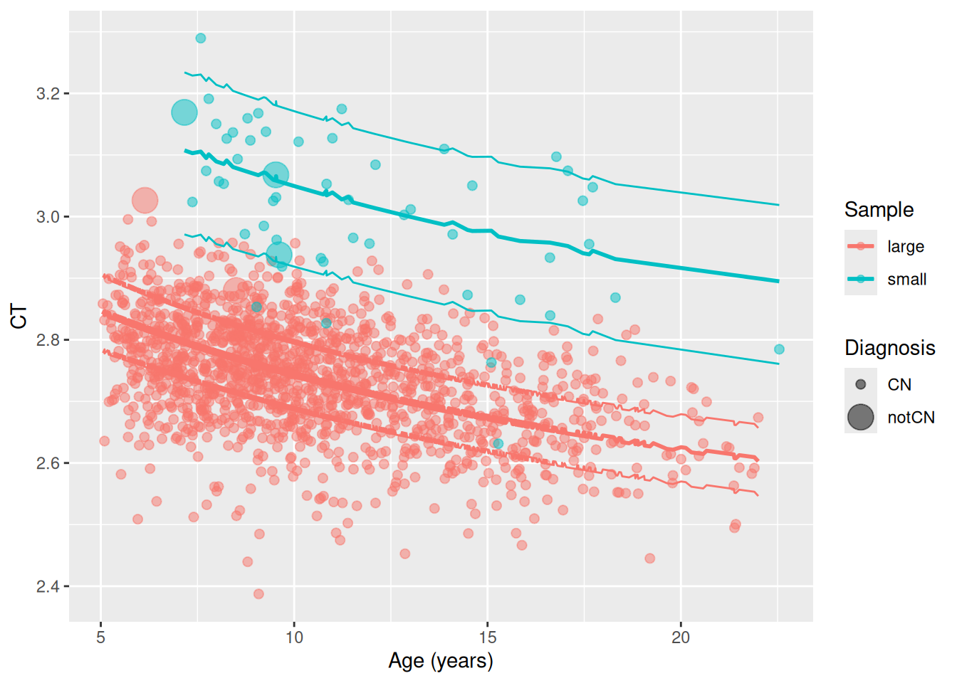
This plot depicts a typical representation of the measured data and the estimated centile lines. The original data are plotted as points with the centile lines overlaid. The implication of the calibration is that data points are to be characaterised by their centiles. Thus, the centiles provide a common frame of reference to compare timepoints between samples that is free of sample biases.
T <- bind_rows(fullSampleCalibration$DATA.PRED2, subFakeQuantileCalibration$DATA.PRED2)
M <- c(CN = 1, notCN = 5)

T$DXSize <- factor(M[T$dx], labels=c("CN", "notCN"))

ggplot(T, aes(x = age_days / 365.25)) +
  geom_point(aes(y = meanCT2Transformed * 10000, colour=sample, size = DXSize), alpha = 0.5) +
  geom_line(aes(y = PRED.l250.wre * 10000, colour=sample)) +
  geom_line(aes(y = PRED.m500.wre * 10000, colour=sample), linewidth = 1) +
  geom_line(aes(y = PRED.u750.wre * 10000, colour=sample)) +
  labs(x = "Age (years)", y = "CT", colour = "Sample", size = "Diagnosis")